
Thanks for attending the META Lab's Introduction to R Geek Out!
We're going to try and cover as much ground as possible in our limited time, but not to the detriment of learning what the code is doing or what its potential applications are.
Do not feel overwhelmed or that you are expected to immediately grasp everything that we cover. Today is a VERY cursory overview of R
Today's intent is not to immediately transform you into a functional programmer. That is not a remotely realistic goal.
Instead, the goal is to provide you with a basic grasp of how R works and some resources and support to puruse further learning.
If you have questions on anything, now or in the future, please feel free to ask. Thanks again for coming!

Ris a language and environment for statistical computing and graphics.Ris an integrated suite of software facilities for:- data manipulation,
- calculation,
- and graphical display.
- The term “environment” is intended to characterize it as a fully planned and coherent system
- as opposed to being an incremental accretion of very specific and inflexible tools.
- Inflexibility frequently characterizes other data analysis software.
- as opposed to being an incremental accretion of very specific and inflexible tools.
- One of
R’s strengths is the ease with which well-designed publication-quality plots can be produced. - Many users think of
Ras simply a statistics system.- It's more accurate to think of it as an environment within which statistical techniques are implemented.
Ris available as Free Software under the terms of the Free Software Foundation’s GNU General Public License.
Takeaway: R is a powerful, free, extensible platform with which you can perform analysis that may not be possible in other platforms.

RStudiois a free and open-source integrated development environment (IDE) forR.- An
IDEis a software application that provides comprehensive facilities to computer programmers for software development.- Think of an
IDEas a really fancy text editor that allows you to write, run, debug, share, and deploy code.RStudiois undoubtedly one of the perks of usingRas likely all of your work can be completed withinRStudio.
- Think of an
- An
Takeaway: RStudio is a powerful, free IDE that offers the ability to perform practically every task of a data science project in one environment.


- Bus Routes: Tracking locations over time using streaming data
- Diagnostics for Lake Erie fisheries
- San Francisco Crime Map, Live Simulation


... and those are just the pretty pictures I found in a few minutes of 5am Google-Fu!
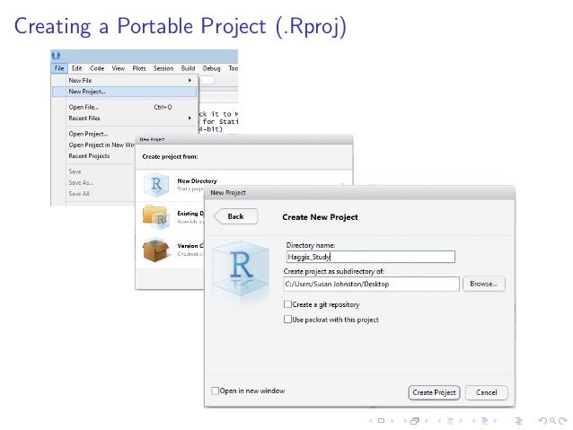
By using RStudio's project manager, we can eliminate many of the common headaches associated with file management.
Keeping our work in a project:
- automatically sets our
working directoryto the project's folder - creates a
.Rprojfile that allows us to easily return to our project - facilitates simple sharing our code, data, and reports
We're going to use R Markdown for our code as it lets us:
- Perform our analysis
- Share our code, workflow, exploration, and findings
- Reproduce our results
- Reproducibility is the ability of an entire analysis of an experiment or study to be duplicated, either by the same researcher or by someone else working independently.
When we're doing any sort of analysis, we want to keep in mind that our data tells a story. R Markdown lets us turn our analyses into professional quality documents, reports, presentations, and dashboards.


RStudio provides some sample code when you open a new .Rmd file, but you can go ahead ad delete everything below the chunk with the following code:
knitr::opts_chunk$set(echo = TRUE)R code chunks can be used as a means render R output into documents or to simply display code for illustration. Another perk is that it allows us to organize our code and thus our analytical workflow.
We're not going to dive into everything that you can do with R Markdown, but here's a cheatsheet that explains much of the syntax that you can use to customize your reports.
For now, just know that you can type explanatory notes between code chunks.
As you can see, code chunks in RStudio are highlighed with a gray background. Everything you put in this chunk will be evaluated by R Markdown as R code when you knit the document.

You can insert a new code chunk in a few ways:
- Click the “insert new code chunk” button on the top right hand of this panel. It looks like a green square with an arrow.
+ Your version may look a bit different
- Copy and paste an existing chunk and change its content and properties.
You may notice that there are setting you can customize for each chunk. Don't worry about that for now, but realize it's there for the future.
Go ahead and insert a new R code chunk.
In order to run your code, you can:
- click the green arrow on the right side of the code
chunk - click
Runat the top of your screen - use Ctrl + Enter/Return to run your current line
- use Ctrl + Shift + Enter to run your current chunk
You're going to see # in this code, which is used to comment within code. R sees # and knows not to try and run execute whatever follows it on the same line.
1 + 2 # addition## [1] 3
2 - 1 # subtraction## [1] 1
3 * 3 # multiplication## [1] 9
9 / 3 # division## [1] 3
3 ** 2 # exponents## [1] 9
9 %% 2 # modulo, which returns the remainder of division## [1] 1
As opposed to many other programming languages, proper R syntax uses <- for variable assignment, rather than the more commonly seen use of = you may have seen in C-based languages like Python.
While using = will variable accomplish the task of assignment without any side-effects in the vast majority of cases, you should stick to the R convention of <- as = there are different uses for each, your code will be more readable to other useRs, the habit will set you up to read the code of other useRs better, and you won't be forced to break the habit in collaborative projects that enforce proper syntax (read: 99% of them).
Think of using proper syntax as being analogous to writing a paper in the proper format. Ensuring that your code is readable should be a priority, even if you will never share it. You will likely encounter challenges that you overcame months earlier. You want to be able to return to your old code and actually understand the solution you used.
On that note, just what the heck is assignment anyways?
When programming, you will want to be able to assign data to variables that you can use in other parts of your code.
x <- 1

x
## [1] 1
y <- 1

z <- x + y

z
## [1] 2
We already saw numerical data above, but we can do a lot more than just numbers.
For characters (commonly referred to as strings), we encapsulate our data with ""
first_name <- "John"
last_name <- "Smith"
We can use numbers as strings too.
one <- "1"

one
## [1] "1"
In that case, what if we aren't sure what type of data is store in a variable?
mode(one)## [1] "character"
a_vector <- c(1, 2, 3)

a_vector
## [1] 1 2 3
We'll use the first_name and last_name variables that we created above.
a_list <- c(first_name, last_name)

a_list
## [1] "John" "Smith"
To compare objects, we often want to evaluate whether an object is equal to another object.
==checks to see if 2 objects are equal to eachother.!=checks to see if 2 objects are not equal to eachother.
1 == 2## [1] FALSE
1 != 2## [1] TRUE
We can also combine our logical evaluations.
&simply meansand, which we can use to evaluate whether 2 (or more!) conditions are bothTRUE. + If either one isFALSE, then the whole expression isFALSE.
1 == 1 & 2 == 2## [1] TRUE
1 == 2 & 2 == 2## [1] FALSE
|meansor, which we can use to evaluate whether or not any conditions areTRUE.
1 == 1 | 2 == 3## [1] TRUE
1 != 1## [1] FALSE
First, let's create a few vectors of data...
a <- c(1, 2, 3)
b <- c(4, 5, 6)
c <- c(7, 8, 3)

a
## [1] 1 2 3
b## [1] 4 5 6
c## [1] 7 8 3
... and we want to combine our vectors into a matrix using rbind()
rbind()simply stands forrow bind, and treats ourvectors as rows in amatrix. For now, think of amatrixas a collection ofvectors.
my_matrix <- rbind(a, b, c)

my_matrix
## [,1] [,2] [,3]
## a 1 2 3
## b 4 5 6
## c 7 8 3
If we look at the mode of my_matrix we see that it is numeric data...
mode(my_matrix)## [1] "numeric"
But there are MANY types of numeric data in R, so we can get more specific by checking its class...
class(my_matrix)## [1] "matrix"
Don't worry about what class is referring to now, but just realize there are ways to figure out which type of data you're dealing with.
Returning to the matrix we already created...
my_matrix## [,1] [,2] [,3]
## a 1 2 3
## b 4 5 6
## c 7 8 3
We can access the third row by using subscripts, i.e. variable[row, ]...
third_row <- my_matrix[3,]

third_row
## [1] 7 8 3
We can do the same to the third column with variable[, column], which also gives us our row names...
third_column <- my_matrix[, 3]

third_column
## a b c
## 3 6 3
Finally, we can access individual values from our matrix by using both row and column subscripting...
bottom_right <- my_matrix[3, 3]

bottom_right
## c
## 3
Make sure you understand that the convention for subscripting then is my_matrix[row,column]
A data.frame is very similar to a matrix in that they are both forms of tabular data containing columns and rows, but there are some differences in their use.
The most important differences for now is that a matrix should
- a
matrixshould contain data that are of the same type, while adata.framecontain mixed types of data data.frames are more general in that different columns can have different types of data- this is what you'll typically see when dealing with data "in the wild"