We have been approached by a real estate company about how to accurately appraise homes in King County so that they can give their customers accurate reccomendations when it comes to buying and selling homes. We've been given a data set that contains various information about the different homes within King County.
We'll be looking to answer the following questions to help us better understand the layout of the housing industry.
- How does number of bathrooms/bedrooms effect the price?
- How much does square footage matter?
- Are there any other features that effect the price significantly?
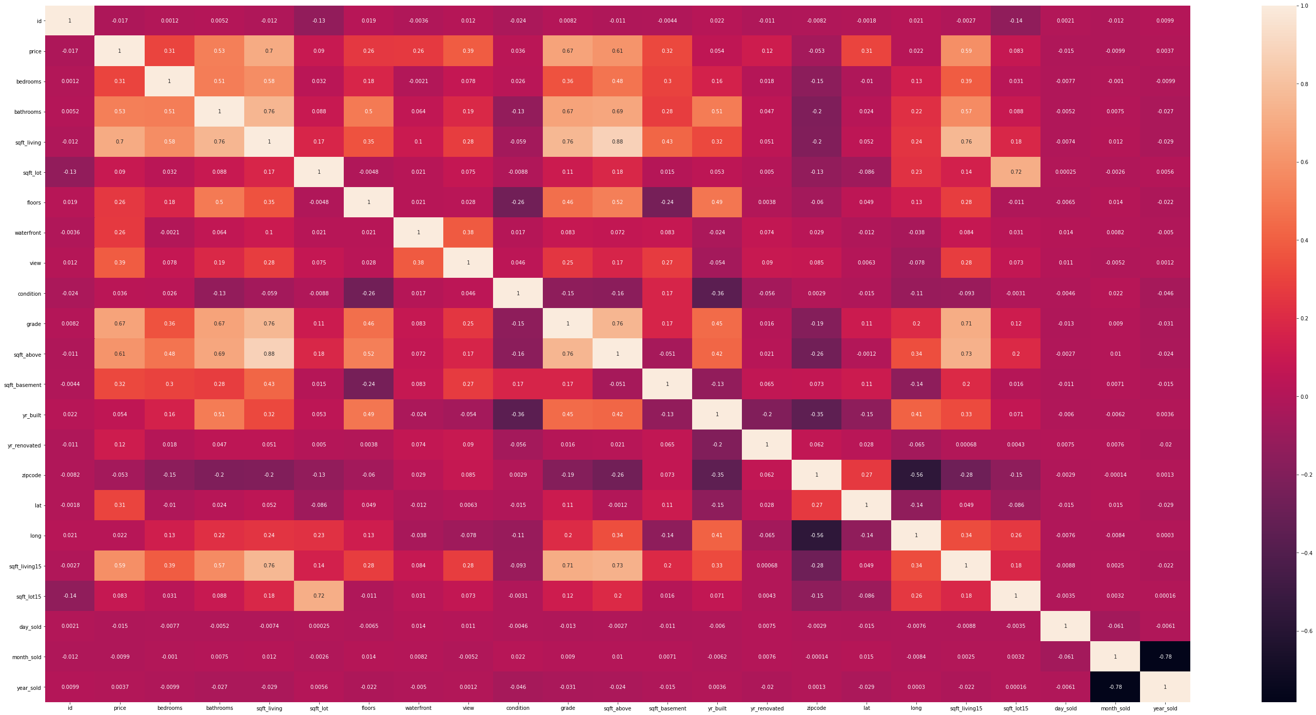 From the heatmap you can see that sqft_living is the most correlated feature so we'll be using that as our baseline model
Train score: 0.48733518973535617
Validation score: 0.4945445156766466
We did linear regression on our baseline model and it showed that our r-squared value is .49.
We will try to make our model better
From the heatmap you can see that sqft_living is the most correlated feature so we'll be using that as our baseline model
Train score: 0.48733518973535617
Validation score: 0.4945445156766466
We did linear regression on our baseline model and it showed that our r-squared value is .49.
We will try to make our model better
We will start by checking linearity between price and independent variables.
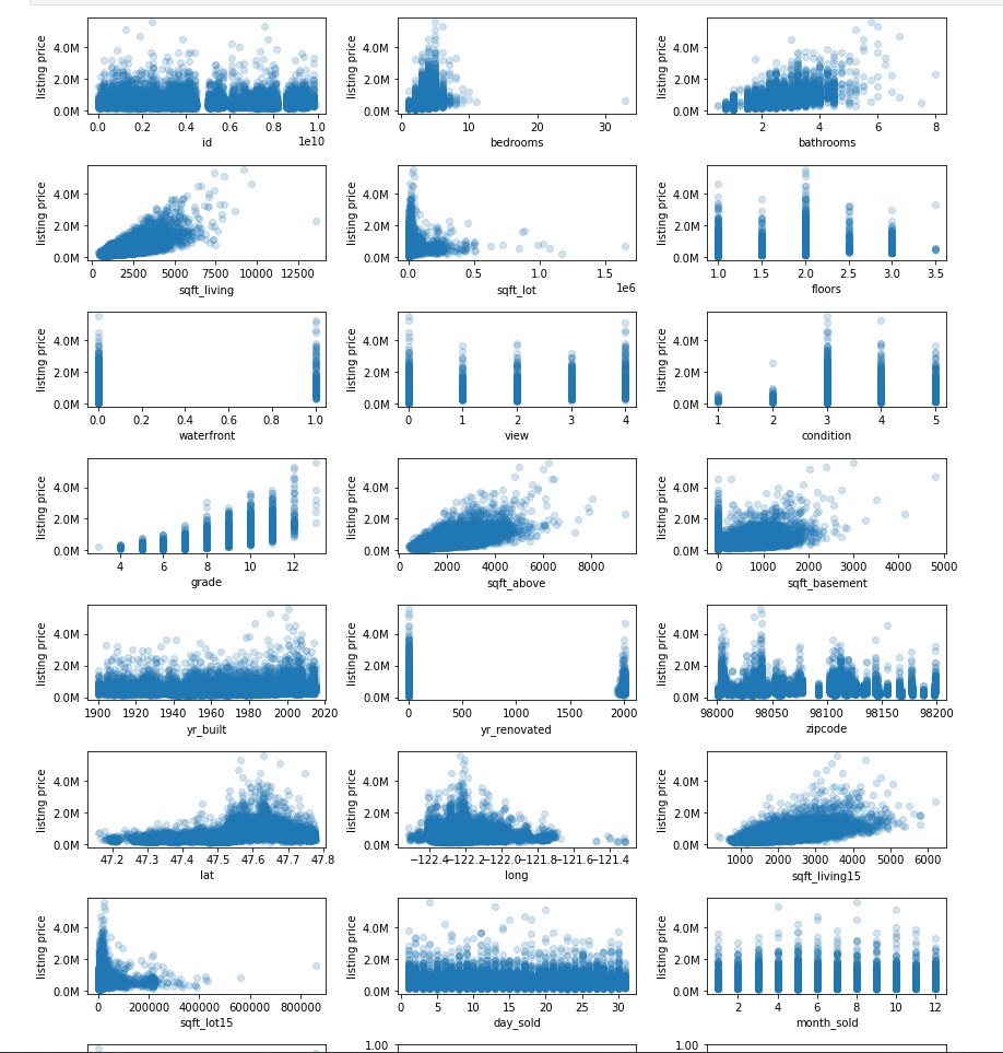
From the above graphs, we can see that the following independent variables have a linear relationship to listing price:
- sqft_living15
- grade
- sqft_above
- sqft_living
- bathrooms
then we'll check for collinearity between independent variabels
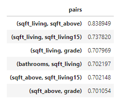
Looks like there's a good amount of collinearity in our data. In order to avoid this we have to drop one variable from each pair. If we dropped sqft_living and sqft_above, we'd be able to keep grade, bathrooms, sqft_living15. We also still have our bedrooms variable, as well as our sqft_basement.
Alternatively though the above collinearity check included outliers in the data set. After putting the columns we were planning to remove after the first collinearity test back into the data and removing outliers we got different results.
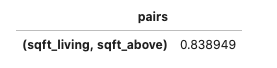
Now, the only colinear factors we found were sqft_living and sqft_above. This allows us to remove sqft_above and keep more columns in our data set than we would have been allowed to do before removing outliers. Now we can model this again and see what we get.
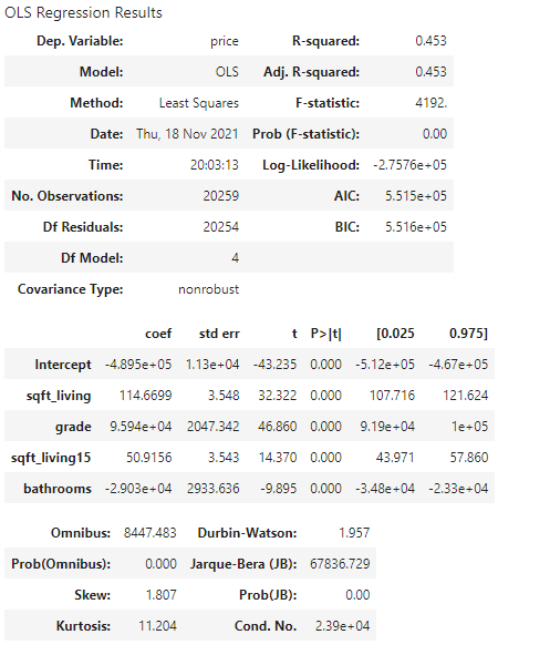
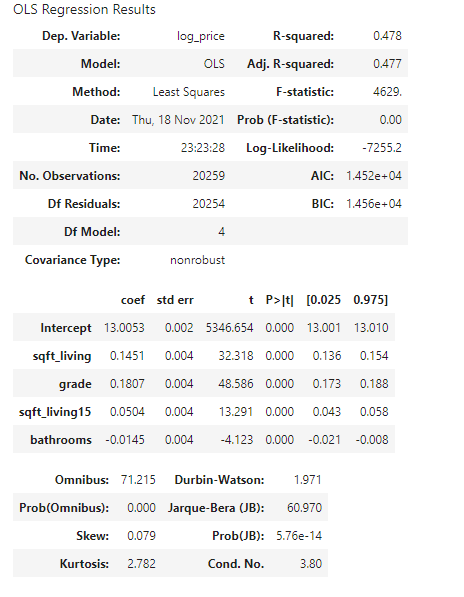
Looking at the coefficients from this model, we can see that the sqft of a home on average will increase the sale price by 114 per square foot, the sqft of the 15 surrounding homes will on average increase the sale price by 50, and improving the grade will increase the sale price by 90,000.
But we know that because grade is really a categorical number rather than a numerical number, all we can really infer from this is that the grade is strongly correlated, but we can't put a specific number on it.
Bathrooms, interestingly enough have a negative correlation. The explanation for this may be, that because the model takes in to acount the square footage, it wants to figure out how bathrooms impact the price given that it's a big home. In that case it is possible that homes that are very big and therefore expensive don't have higher prices when there are more bathrooms.
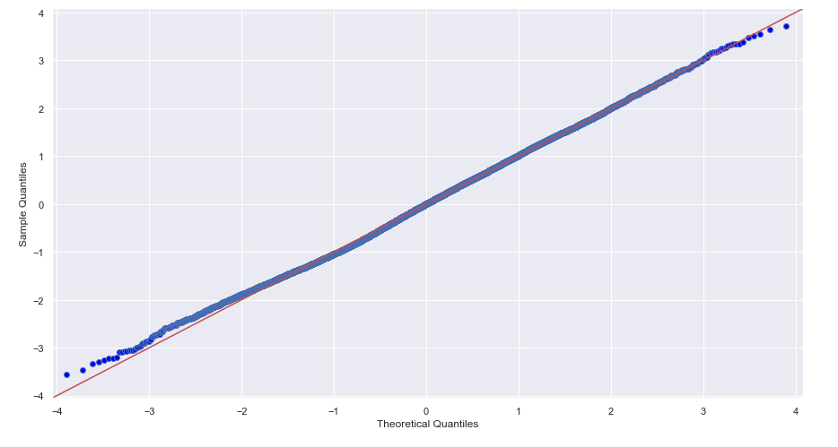
Investigating Normality
Regression Plots
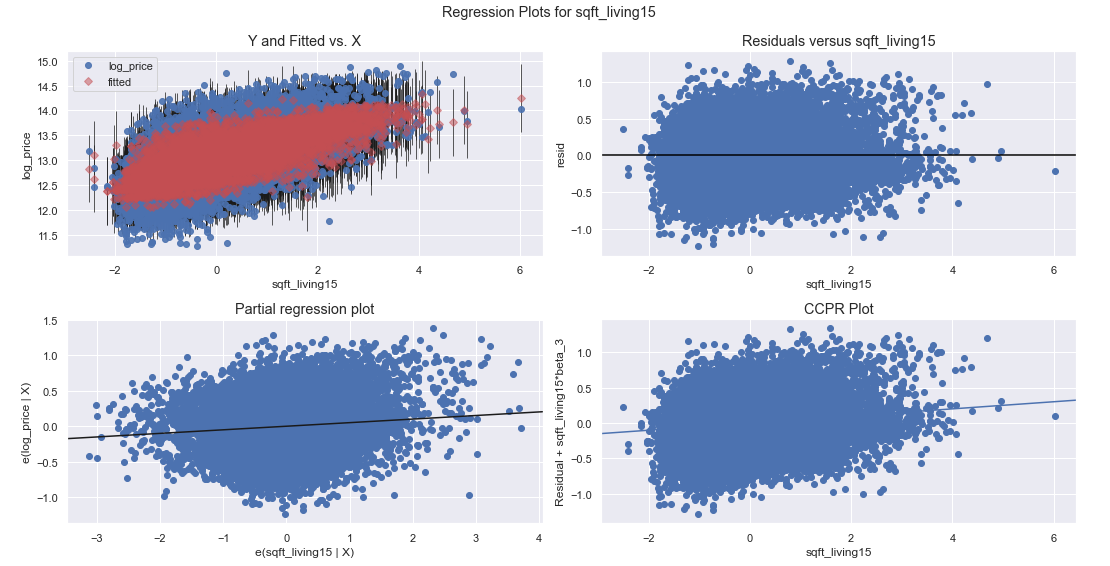
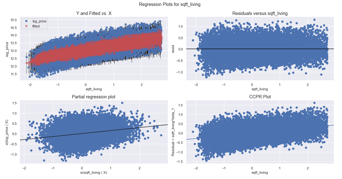
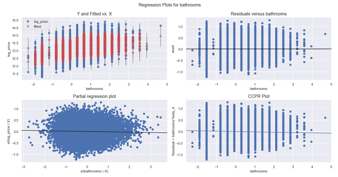
This is how we'd expect our final model to perform. The RMSE matches the same RMSE as our fourth model HOWEVER we made these changes to the final model to satisfy the assumptions of linear regression. The four independent variables are homoscedastic by the graphs above meaning the variance doesn't increase as the independent variable gets bigger or smaller. We also know that these aren't collinear given the correlation graph we used above.
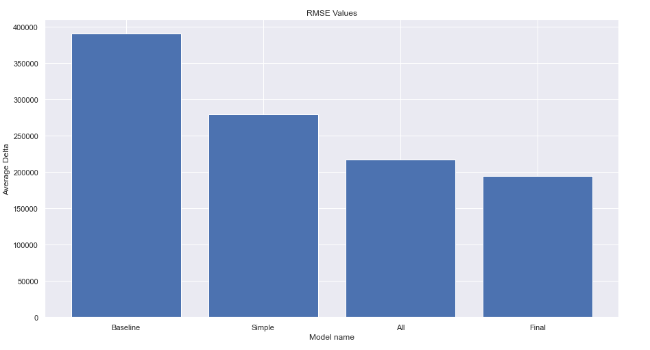
After analyzing this King County data, our final model would suggest the main factors in increasing property value to be sqft of the property as well as it's grade. Grade is referring to the classification based on a structures construction quality. This mainly has to do with the types of materials used and the quality of the work done. Buildings that get better grades often cost more to build per unit of measure howevever we deem that investment profitale as properties that do grade higher, command higher value. Our model does however have it's faults. Our final models R^2 was 48% with an RMSE of $194,053. Linear regression was probably not the best tool to use to get the most out of this data set so in the future we would like to use different more powerful machine learning tools in order to make this a more accurate predictive model.